(著)山たー
MatlabやRでは線形回帰のモデルをfitして以下のように結果を表示してくれるライブラリがある。
R
> sample=read.csv("boston_housing_data.csv")
> model=lm(Y~., data=sample)
> summary(model)

Call:
lm(formula = Y ~ ., data = sample)

Residuals:
     Min       1Q   Median       3Q      Max
-15.5795  -2.7256  -0.5165   1.7831  26.1887

Coefficients:
              Estimate Std. Error t value Pr(>|t|)
(Intercept)  3.649e+01  5.104e+00   7.149 3.18e-12 ***
CRIM        -1.072e-01  3.271e-02  -3.276 0.001126 **
ZN           4.640e-02  1.373e-02   3.380 0.000784 ***
INDUS        2.086e-02  6.150e-02   0.339 0.734597
CHAS         2.689e+00  8.616e-01   3.120 0.001912 **
NOX         -1.780e+01  3.821e+00  -4.658 4.12e-06 ***
RM           3.805e+00  4.180e-01   9.102  < 2e-16 ***
AGE          7.511e-04  1.321e-02   0.057 0.954686
DIS         -1.476e+00  1.995e-01  -7.398 6.02e-13 ***
RAD          3.057e-01  6.633e-02   4.608 5.19e-06 ***
TAX         -1.233e-02  3.761e-03  -3.278 0.001118 **
PTRATIO     -9.535e-01  1.308e-01  -7.287 1.27e-12 ***
B            9.392e-03  2.684e-03   3.500 0.000507 ***
LSTAT       -5.255e-01  5.069e-02 -10.366  < 2e-16 ***
---
Signif. codes:  0 ‘***’ 0.001 ‘**’ 0.01 ‘*’ 0.05 ‘.’ 0.1 ‘ ’ 1

Residual standard error: 4.746 on 492 degrees of freedom
Multiple R-squared:  0.7406,    Adjusted R-squared:  0.7338
F-statistic: 108.1 on 13 and 492 DF,  p-value: < 2.2e-16
Matlab
mdl =

線形回帰モデル:
    y ~ 1 + x1 + x2 + x3 + x4 + x5 + x6 + x7 + x8 + x9 + x10 + x11 + x12 + x13

推定された係数:
                    Estimate        SE         tStat        pValue
                   __________    _________    ________    __________

    (Intercept)        36.491       5.1045      7.1488    3.1824e-12
    x1               -0.10717     0.032712     -3.2762     0.0011264
    x2               0.046395     0.013728      3.3796    0.00078361
    x3                0.02086     0.061497     0.33921        0.7346
    x4                 2.6886      0.86162      3.1204     0.0019123
    x5                -17.796       3.8206     -4.6579    4.1173e-06
    x6                 3.8048        0.418      9.1023    2.2075e-18
    x7             0.00075106     0.013211    0.056852       0.95469
    x8                -1.4758      0.19948     -7.3979    6.0177e-13
    x9                0.30566     0.066333      4.6079    5.1897e-06
    x10             -0.012329    0.0037608     -3.2784     0.0011178
    x11              -0.95346      0.13084     -7.2872    1.2682e-12
    x12             0.0093925    0.0026835      3.5001    0.00050729
    x13              -0.52547      0.05069     -10.366    6.5958e-23


観測数: 506、誤差の自由度: 492
平方根平均二乗誤差: 4.75
決定係数: 0.741、自由度調整済み決定係数 0.734
F 統計量と一定のモデルの比較: 108、p 値は 6.95e-135 です
これを表示するプログラムをPythonで書いてみる。
ソースコード
import numpy as np
import pandas as pd
from sklearn.datasets import load_boston
import scipy as sp

#データを計画行列に変換
def make_design_matrix(X,n):
    return np.concatenate([np.ones((n,1)), X], axis=1)

#正規方程式を解いて係数の推定値を計算
def estimate(X,y):
    return np.linalg.inv(X.T @ X) @ X.T @ y

#残差を計算
def residual_error(X,y):
    residual = y - estimate(X,y) @ X.T
    return residual

#標準誤差(standard error)
def St_Error(X,y,n,p):
    #残差を計算
    residual=residual_error(X,y)
    #残差平方和Sを計算
    S=np.sum(residual.T @ residual)
    #推定値の分散を計算
    var_estimate=(1/(n-p-1))*S*np.linalg.inv(X.T @ X)
    #対角成分を取って平方根を取る
    StdE=np.sqrt(np.diag(var_estimate))
    return StdE

#t値
def t_value(estimate, StdE):
    return estimate/StdE

#p値
def p_value(t,n,p):
    return 2*(1-sp.stats.t.cdf(np.abs(t),n-p-1))

#線形回帰
def linearMod(X,y,n,p):
    Xd=make_design_matrix(X,n)
    beta=estimate(Xd,y)
    StdE=St_Error(Xd,y,n,p)
    tValue=t_value(beta,StdE)
    pValue=p_value(tValue,n,p)
    matrix=np.concatenate([beta, StdE,tValue,pValue], axis=0)
    matrix=np.reshape(matrix,(4,p+1)).T
    indexlist=['(Intercept)']
    indexlist.extend(['x'+str(i) for i in range(1,p+1)])
    df=pd.DataFrame(matrix,
                    index=indexlist,
                    columns=('Estimate', 'Std. Error','t value','Pr(>|t|)'))
    return df

#Boston Housing Dataをインポート
boston = load_boston()
X=boston.data
y=boston.target
n=X.shape[0] #サンプル数
p=X.shape[1] #説明変数の数

#線形モデルにfit
model=linearMod(X,y,n,p)

#結果表示
print('Coefficients:')
print(model)
結果
Coefficients:
              Estimate  Std. Error    t value      Pr(>|t|)
(Intercept)  36.491103    5.104500   7.148811  3.182565e-12
x1           -0.107171    0.032712  -3.276202  1.126402e-03
x2            0.046395    0.013728   3.379596  7.836070e-04
x3            0.020860    0.061497   0.339209  7.345971e-01
x4            2.688561    0.861617   3.120369  1.912339e-03
x5          -17.795759    3.820585  -4.657862  4.117296e-06
x6            3.804752    0.417998   9.102313  0.000000e+00
x7            0.000751    0.013211   0.056852  9.546859e-01
x8           -1.475759    0.199483  -7.397902  6.017409e-13
x9            0.305655    0.066333   4.607863  5.189664e-06
x10          -0.012329    0.003761  -3.278408  1.117826e-03
x11          -0.953464    0.130841  -7.287219  1.268097e-12
x12           0.009393    0.002683   3.500142  5.072875e-04
x13          -0.525467    0.050690 -10.366343  0.000000e+00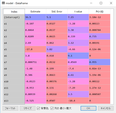
他の部分は次の機会につくる。
コメントをお書きください